Why Discriminant Analysis Still Dominates Predictive Targeting

The Insight Industry’s Go-To Tool for Segment Reclassification and Scalable Precision Marketing

In the world of data-driven marketing, knowing your segments is only half the battle. The real value comes from reclassifying, scaling, and predicting—turning insight into action. That’s where discriminant analysis earns its reputation as the most commonly used technique in the insights industry for reclassification of existing segments.

Unlike exploratory tools such as cluster analysis, discriminant analysis starts with what many real-world marketers already have: defined customer groups. The power of the method lies not just in explaining what differentiates those groups—but in its ability to predict future membership with precision, even from a few key inputs. This makes it a cornerstone in survey analytics, segmentation follow-up, and targeted messaging strategies.

From brand trackers to B2B segmentation to churn models, discriminant analysis has become a go-to modeling framework for predictive analytics, giving marketers, strategists, and insight professionals a clear and repeatable path from raw survey data to qualified leads and scalable strategies.

Discriminate analysis is a statistical technique used to differentiate between two or more predefined groups, based on a set of independent variables. In this case, our goal was to discriminate between members of a high-value customer segment and everyone else—based on characteristics like attitudes, perceptions, and firmographics.

The output of a discriminant analysis is a linear function—or a set of functions, in the case of multiple groups—that assigns weights to each predictor. This scoring equation can be used in two powerful ways: (1) to classify new respondents into the most likely segment, or (2) to understand which variables are doing the heavy lifting in separating the groups.

This often gets confused with cluster analysis, which is also used in segmentation. But the logic runs in the opposite direction. In cluster analysis, you start with raw data and let the algorithm create the segments. In discriminant analysis, you already have the segments—you’re figuring out what defines them.

Step One: Define the Target

Discriminant analysis is an a priori method. That means group membership needs to be known in advance—distinct, mutually exclusive, and exhaustive. For our client’s purposes, we recoded respondents: 1 for those in the target segment, 0 for all others.

No fuzzy boundaries here. The algorithm assumes clean input on group identity.

Step Two: Choose the Right Predictors

Now comes the part that blends statistical rigor with marketing intuition: selecting predictor variables. These need to be independent (or at least not collinear), and ideally normally distributed. But they also need to make sense from a business perspective.

In this case, we had plenty of options: perceptions of technical capability, customer service ratings, brand image, firm size, revenue, geographic region, and more. But more data isn’t always better. Overloading the model with too many inputs can lead to noise, overfitting, and a lack of interpretability.

Instead, we worked with the client to narrow the focus to five predictors with clear marketing value: perceived technical expertise, quality of marketing support, customer service ratings, firm size, and revenue. These variables not only performed well statistically—they were actionable.

From Math to Market Targeting

With that model in hand, the client’s team was able to run discriminant scores in subsequent surveys and re-identify their high-likelihood, low price-sensitivity audience. Better yet, they could now build lookalike strategies, retarget campaigns, and refine messaging based on the drivers that mattered most.

Basics of Discriminant analysis

Discriminant analysis is an apriori technique. The first requirement, then, are the groups. You need to have groups defined. Multiple discriminant analysis, from which discriminant maps are drawn, is a case when you have membership from more than one group to define. In this article, for the sake of easy understanding of the technique, we are going to restrict our case to two groups.

Characteristics of the grouping variable are simple. They are distinct, mutually exclusive, and exhaustive. In the case of my client’s request, either a respondent is in the target group, or he isn’t. No fence sitting. No overlapping. To conduct the discriminant analysis, I recoded the segmentation into 1 for ‘Group Members’ and 0 for ‘Non-Group Members’.

Basic data assumptions of the predictor variables are normally distributed and independent.

Choosing which predictor variables will be included in the analysis requires a bit of marketing sense. For example, our client seeks to distinguish between high probability clients and low-probability clients. Within the survey respondents are asked to rate the company on a given array of rankings of importance, performance, and company image, demographics, such as size of respondent firm, revenue, number of employees, and geographic area. A good analysis, especially if it is going to be used for back classification, cannot use all the data available. The results would be murky and there would be a good deal of variation error, commonly referred to as ‘noise’.

Therefore, it is vital to choose which predictors go into the equation. Aside from the actual data processing, Multivariate Solutions specializes in advising our clients as to the marketing actionability of the results. In our fictitious example, similar to the case above, attitudes of the technical prowess of the client, marketing support, customer service, size of firm, and revenues were chosen.

Discriminant Analysis: The Essentials

Discriminant analysis is a supervised technique used to classify cases into predefined groups based on predictor variables. Unlike cluster analysis, which forms groups from scratch, discriminant analysis starts with known categories—like high- vs. low-value customers—and builds a model that best separates them.

Clear Group Definitions

The foundation of discriminant analysis is a grouping variable. Each observation must belong to a distinct, mutually exclusive, and exhaustive group. For binary classification, we typically assign a 1 (target group) or 0 (non-target). This structure allows the model to calculate which variables most effectively distinguish between the groups.

Key Assumptions

· The model assumes:

· Normality of predictors within each group

· Equal variance-covariance matrices (for linear models)

· No multicollinearity among predictors

· Independence of observations

Violating these assumptions can reduce the model’s reliability. It’s best to test data quality in advance using checks like Box’s M and correlation matrices.

Selecting Predictors

Not all variables belong in the model. Including too many inputs can muddy results and introduce noise. Choose predictors based on relevance and distinctiveness—such as technical satisfaction, service perception, firm size, and revenue. Pairing subject-matter insight with statistical screening helps ensure the final model is both interpretable and predictive.

The Discriminant Function

The result is a linear function: D = b₀ + b₁x₁ + b₂x₂ + ... + bₖxₖ

Here, x’s are predictor values and b’s are weights derived from the data. Each case receives a score, which is compared to a cutoff point to determine group membership. The model can then be validated using metrics like classification accuracy and Wilks’ Lambda, which tests whether group separation is statistically meaningful.

Real-World Use

Once built, the function isn’t just explanatory—it’s predictive. You can apply it to new data to score and classify future cases. Marketers, for example, can use it to identify high-value prospects in ongoing surveys and target them more precisely.

In short, discriminant analysis offers a structured way to turn existing groups into actionable insights. When done right, it enhances targeting, segmentation, and strategic decision-making.

Let me know if you'd like this version adapted into a slide deck, executive summary, or included in a client-

The Output

The analysis produces a discriminant function—a linear equation in which coefficients are multiplied by the values of the predictor variables to generate a discriminant score. Based on this score, the likelihood of group membership is calculated using prior group classifications.

As with all advanced statistical procedures, the output includes a flurry of diagnostics. For a Ph.D. statistician from MIT, these are fascinating. For a consultant, they’re useful for evaluating model viability. But for the end user—the client—the key question is: What should we actually be looking at?

There are five core outcomes I examine and report:

1. The raw (beta) coefficients of the discriminant function

2. The standardized coefficients

3. Wilks’ Lambda

4. The discriminant score

5. The percentage of correctly reclassified respondents

The raw and standardized coefficients are used primarily for descriptive insight and understanding variable contribution, which I’ll elaborate on below. The discriminant score, once calculated, becomes the operational tool for future classification.

Wilks’ Lambda measures the strength of the model; if its associated chi-square test is statistically significant, the model can be considered robust. Lastly, the reclassification rate tells us how accurately the model assigns respondents back to their original groups—an essential indicator of predictive power.

The Analysis—Descriptive Aspects

Once the groups are defined (e.g., potential clients vs. non-potential clients), the predictor variables are selected, properly recoded, and the analysis is executed. To make the results more digestible and actionable, we often transfer key findings into Excel spreadsheets or PowerPoint slides. These are presented in exhibit tables—formats that are easy for clients to interpret and incorporate into their own reporting.

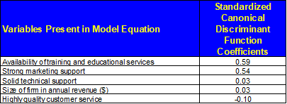
Figure 1 below presents the standardized discriminant coefficients in Excel format.

Figure 1 – Discriminant Analysis: Standardized Descriptive Coefficients

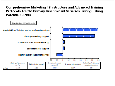
Figure 2 presents a visualization of the relative impact of each attribute in identifying potential clients, referred to as key discriminators.

Figure 2 – Discriminant Analysis: Visualization Key Drivers of Potential Clients

From this point, I will walk through the example as I would present it to a client. The first output I typically share—primarily for descriptive purposes—is the set of standardized coefficients.

When interpreting standardized coefficients, their relative size is more informative than their absolute value. For example, Availability of Training and Educational Services has a coefficient of 0.590, while Strong Marketing Support follows closely at 0.537. These two are clearly the strongest indicators of group membership. By contrast, Solid Technical Support (0.032), Size of Firm in Annual Revenue (0.032), and High Quality Customer Service (-0.103) have coefficients close to zero, indicating weak discriminatory power.

As a rule of thumb: if one predictor’s standardized coefficient is twice that of another, it is approximately twice as effective at distinguishing group membership. While weak predictors contribute little, they must remain in the classification equation for reclassification purposes.

From a marketing standpoint, the implications are straightforward. Technical support, company size, and customer service play only a minor role when clients evaluate potential vendors. Instead, Marketing Support and Training emerge as the most actionable differentiators and primary drivers of customer potential. Although this conclusion is statistically supported by the model, it aligns intuitively as well: if a respondent perceives the company as offering strong training and marketing support, they are far more likely to be a viable customer.

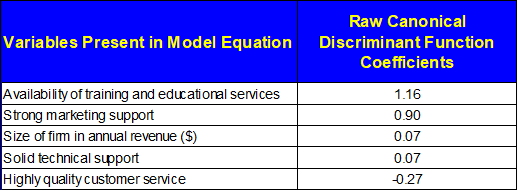
The following chart presents the raw coefficients, which are used to compute the actual discriminant scores for predictive classification.

Figure 3 – Discriminant Analysis – Raw Coefficients

Raw coefficients can also be interpreted descriptively, though I primarily rely on standardized coefficients for that purpose. This is because standardized coefficients adjust for the differing scales of predictor variables—each is normalized to have a mean of 0 and a standard deviation of 1—making direct comparisons meaningful. In contrast, raw coefficients serve a dual role: they are both descriptive and operational, as they are used to generate predictive scores in the classification phase.

It’s also important to evaluate the overall model performance. In the initial output, we see Wilks’ Lambda and the percentage of cases correctly reclassified. In our example, Wilks’ Lambda is statistically significant. For practical interpretation, we look at the associated Sig. value, which reflects the probability that the model has no predictive power. A Sig. of 0.000 means there is virtually no chance the model is meaningless. As a general guideline, I consider any model with a Wilks’ Lambda significance below 10% to be acceptable.

With 67.4% of respondents correctly reclassified, this model demonstrates strong predictive accuracy and can be considered a good fit for the segmentation task at hand.

The Analysis—Predictive Aspects

At this stage, the client’s goal is typically twofold: (1) to reclassify respondents in future studies using the existing group definitions, and (2) to apply the model in a practical setting—such as a sales call—by asking a few key questions and determining whether a potential customer is likely to belong to the target group. To support these objectives, three related functions are used in tandem.

First, a critical point: for the reclassification to work accurately, you must ask the exact same questions used in the original model, and on the same scales. Any variation will compromise the integrity of the results.

The reclassification process is straightforward. Ask the model’s predictor questions, input the responses into the equation, and calculate the discriminant score. For large-scale applications, Multivariate Solutions provides an SPSS syntax script that automates this process—generating banner points and reassigning respondents into the appropriate categories.

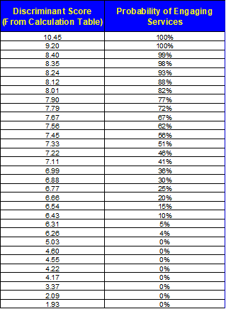
For individual-level predictions, we build a simple Excel-based calculator. The next figure displays this tool in action. It works by calculating the respondent’s discriminant score and then matching it against predefined values in a lookup table. In our example, the respondent yields a score of 7.77.

Figure 4 – Calculation of Discriminant Scores Using Respondent Inputs and Raw Coefficients

We go to the table and find that this score corresponds with a likelihood between 67% and 72% to belong to our target group.

Figure 5 – Discriminant Analysis Lookup Table: Indexed Scores with Percentage Likelihood of Client Interest

In an age dominated by AI and advanced analytics, it's easy to overlook the tools that have quietly driven industry results for decades. Discriminant analysis remains the backbone of predictive segmentation—precise, transparent, and widely adopted in the insights community for a reason.

Its strength lies in operational simplicity and statistical rigor. When used correctly, it can reclassify respondents across waves, score new data on the fly, and—most importantly—tell you which attributes actually matter. It's not just about modeling the past. It's about predicting the future of your customer base.

With powerful applications ranging from custom dashboards to SPSS macros and Excel scoring calculators, discriminant analysis lets clients go beyond analytics and into execution. If someone scores high on “training” and “marketing support,” they’re not just a statistic—they're your next high-value customer.